
Exploring The Sound of Seattle Birds with Neural Networks
Table of Contents
- Table of Contents
- Abstract
- Introduction
- Theoretical Background
- Methodology
- Computational Results
- Discussion
- Conclusion
- References
Abstract
In this report, neural networks are employed to identify the bird species of Seattle. We used spectrograms that were derived from Xeno-Canto’s Birdcall competition dataset that consists of 10 high-quality MP3 sound clips for each of the 12 selected bird species[1]. Additionally, three MP3 bird call recordings were available for external testing. The primary goal is to classify bird species based on their distinct vocalizations. We developed two custom neural network models: a binary classification model distinguishing between the American Crow and the Blue Jay, and a multi-class classification model capable of identifying any of the 12 bird species. Predictions on the three external test clips are made to assess the effectiveness of the models. Neural Networks with different architectures and parameters were employed to find the most efficient model.. For hidden layers, various activation functions such as Relu, SoftMax, or Leaky Relu were used. The report concludes with a discussion on alternative modeling approaches and the suitability of neural networks for this specific application.
Introduction
In this study, a neural network is employed to categorize bird species using pre-processed spectrograms of their sounds. The dataset, originating from Xeno-Canto’s Birdcall competition, comprises original sound clips recorded in the Seattle area. Each clip has been preprocessed into spectrograms, which act as visual representations of the bird sounds and serve as the primary input to the neural networks. These spectrograms are organized in HDF5 format.
The main objective is to develop a robust neural network which can accurately predict species based on their unique sound patterns. We have performed binary as well as multi-class classification tasks on the dataset. We developed various neural network models for the binary classification task to distinguish between the American Crow and the Blue Jay. We used a convolutional neural network for the multi-class classification task that is capable of identifying any of the 12 bird species namely American crow, Barn swallow, Black-capped chickadee, Blue jay, Dark-eyed junco, House-finch, Mallard, Northern flicker, Red-winged blackbird, Stellar’s jay, Western meadowlark, White-crowned sparrow. We have also done a comparative analysis of diverse network structures and hyperparameters to identify the most suitable and efficient model for these kind of classification tasks.
The limitations are discussed in detail for each classification task. Automatic species classification of birds from their sounds has many potential applications in conservation, ecology and archival [2]. The findings of this study can not only help in understanding their unique behavior but also serve as a tool for monitoring bird population and maintaining diversity.
Theoretical Background
Neural networks gained popularity in the late 1980s but they didn’t dominate due to their complexity and also the emergence of simpler methods like SVMs. Few years later, with high computational ability and the availability of huge training datasets eventually led to the rise of neural networks under the new name “deep learning.”[3] Neural networks are machine learning algorithms that resemble the structure and functioning of the human brain. They detect complex patterns in data and forecast outcomes based on these patterns. Neural networks as the word suggests are a network of interconnected nodes like the neurons of our brain, they process information in a layered structure and each node passes the information to the next layer of nodes that it is connected to.
Consider the neural network illustrated in Figure 1 as an example. It consists of three layers: an input layer, a hidden layer, and an output layer. The input layer comprises nodes representing four features, namely x1, x2, x3, and x4. There are five activation functions denoted as A1, A2, A3, A4, and A5. These activation functions can be selected from a range of options such as Relu, tanh, sigmoid, softmax, and others. The choice of activation function depends on the specific objectives of the model and the performance characteristics of each function. Careful consideration is necessary to determine the most suitable activation functions for the desired outcomes.
The input layer receives raw data. The output layer is responsible for making the final predictions. The intermediate levels are known as hidden layers, and they perform intermediary calculations. A neural network adjusts the weights between neurons during training to increase its prediction accuracy. The network is fed a set of labeled training data, and an optimization method is used to update the weights such that the network’s predictions are as close to the true labels as possible.
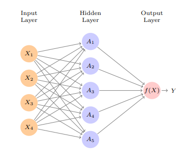
Figure 1 Neural Network with 3 layers- Architecture
For instance, the Rectified Linear Unit, or ReLU, a popular activation function used in neural networks. It works like this:
f(x) = max(0, x); where x is the input.
Essentially, ReLU outputs the input value if it’s positive and outputs 0 if it’s negative. This simplicity makes ReLU both computationally efficient, easy to understand and implement. However, it has a potential downside: sometimes, a neuron might always output 0, becoming what we call a ‘dead neuron’.[4] This can happen if the weights are set in such a way that the neuron always receives negative values. To address this, we can use a variation called Leaky ReLU, which allows a small negative slope, keeping the neuron active even with negative inputs.
Neural networks have many applications like image recognition, natural language processing, and speech recognition. They are highly effective at tackling complex problems that traditional algorithms struggle with. Although they can be quite demanding in terms of the computational power and amount of data that is required for training them.
While training a neural network, there are two important things: the optimizer and the loss function. The optimizer decides how weights and biases of the network are adjusted based on the calculated gradients of the loss function. Its goal is to minimize the loss which in turn guides the network to improve its performance. There are various optimizers to choose from, such as Stochastic Gradient Descent (SGD), Adam, RMSprop, and Adagrad, each with unique characteristics and update rules.
On the other hand, the loss function measures the gap between the neural network’s predicted output and the actual output. It measures how well the network is performing on a specific task. Different tasks, like binary classification, multi-class classification, or regression, require different loss functions. For instance, binary cross-entropy works well for binary classification, categorical cross-entropy for multi-class classification, and mean squared error (MSE) for regression tasks.
Convolutional Neural Networks (CNNs) are a specialized type of deep learning model, commonly used for computer vision tasks such as image recognition and classification. CNNs are designed to automatically learn and extract meaningful features from images, making them perfect for handling large volumes of visual data.
At a high level, a CNN is made up of several layers that transform an input image into an output prediction. The first layer usually performs a convolution operation, applying a set of filters to the input image to extract basic features like edges and corners. Subsequent layers might perform pooling operations to downsample the image and reduce its size. This is then followed by additional convolution layers to extract higher-level features. The final output layer then makes a prediction based on the features extracted from the input image.
A pooling layer helps reduce the size of a large image, condensing it into a smaller, summarized version. A common method used is max pooling. It works by summarizing each non-overlapping 2 × 2 block of pixels in an image, using the maximum value within each block.
For example, max pooling looks at each 2 × 2 block and picks the highest value to represent the entire block. This then reduces the size of the image by a factor of two in each direction, significantly lowering the computational load. Additionally, it also provides location invariance: as long as there is one large value within a block, the whole block is represented by that value in the reduced image. The example below explains max pooling in a simpler way.
Input matrix:
[ 1 2 5 3 ]
[ 3 0 4 2 ]
[ 2 1 3 4 ]
[ 1 1 2 0 ]
After max pooling:
[ 3 5 ]
[ 2 4 ]
CNNs have a great ability to learn features automatically, eliminating the need for manual feature extraction. This makes them highly adaptable to a wide range of tasks, from simple image recognition to more complex tasks like object detection and segmentation. Additionally, CNNs can be trained on large datasets, enabling them to learn highly accurate representations of complex visual patterns.
Methodology
This research aimed to classify bird data into multiple species using an already preprocessed version of Xeno-Canto’s Birdcall competition dataset.[1] This dataset contained raw audio recordings of bird sounds from 12 distinct species. The recordings were in MP3 format, with varying sampling rates and lengths. The methodology used for pre//processing the sound clips to extract bird calls of a specific species involved several steps. Firstly, the sound clip was subsampled to half its original sample rate, resulting in a new sample rate of 22050 Hz. This step is performed to reduce the computational complexity of subsequent processing steps. Secondly, the “loud” parts of the sound clip are identified, specifically those that are greater than 0.5 seconds in duration. From these identified sections, two second windows of sound are selected where a bird call is detected. These windows are then used to extract the relevant bird call data. To further analyze the bird calls, a spectrogram is produced for each 2-second window. The spectrogram provides a visual representation of the sound in terms of its frequency and intensity over time, resulting in a 343 (time) x 256 (frequency) “image” of the bird call. The spectrograms were labeled with the respective bird species names and saved in an HDF5 file, allowing efficient data access and organization for training and testing purposes.
The dataset was divided into training and test subsets to facilitate model evaluation. Eighty percent of the labeled spectrograms were used for training, while the remaining 20% were allocated to the test set. This ensured that the neural network models could learn from a significant portion of the data while being assessed for their ability to generalize on unseen samples. To allow faster convergence, the standard scaler method was applied to the entire dataset to perform data scaling. The dataset was then trained using various neural networks with multiple hidden layers, and the performance of each model was recorded.
This preprocessing methodology provided well-structured spectrogram data, making it suitable for neural network classification and prediction tasks. For binary classification of American Crow and Blue Jay, we built models with different activation functions for the hidden layers such as ReLu, Leaky ReLu, and Sigmoid. Different activation functions affect the rate at which a network learns. Convolutional Neural Network model was also used with and without dropout regularization and different batch sizes were implemented to train the model. This approach was used to find a suitable and efficient model for this kind of classification task. Similarly, for the multi-class classification, we have implemented a CNN with and without dropout regularization, ReLU(hidden layers) and softmax activation function(output layer).
To improve the model’s performance, several dense layers were then added, each consisting of interconnected neurons. These layers serve as the main processing units of the neural network. The first dense layer contains 32 neurons and uses the Rectified Linear Unit (ReLU) activation function, which helps the model learn complex patterns and relationships in the data. A dropout layer was included after the first dense layer to prevent overfitting, a phenomenon where the model becomes too specialized in the training data and performs poorly on new, unseen data.
To further enhance the model’s performance, additional dense layers with 64 and 128 neurons were added, using ReLU activation and dropout regularization. These layers enable the model to learn more intricate features and capture important characteristics of the input data.
The final layer of the model, called the output layer, is responsible for making predictions. It consists of a number of neurons equal to the number of classes in the dataset. In our case, since we are working with categorical data, the output layer uses the softmax activation function, which calculates the probabilities of each class and assigns the input image to the most probable category.
To train the model, an optimization algorithm called Adam was employed. It adjusts the model’s internal parameters to minimize the error between predicted and actual values. The categorical cross-entropy loss function was chosen to measure the dissimilarity between the predicted class probabilities and the true class labels. The model’s performance was evaluated using the accuracy metric, which indicates how well the model correctly predicts the class of the input images. We have also used early stopping to avoid over learning in the model.
For external testing, we preprocessed three MP3 files using the same methodology that was used for the input data. This allowed for uniformity in input data that the model was trained on. A total of 183 spectrograms were obtained from the test MP3 files. Each file was separately fed to the multi-class CNN classification model to make predictions. The spectrograms were also padded to have the same frequency and time dimensions as the training data.
Computational Results
| Activation Function (Hidden layers) | Hidden Layers | Dropout Regularization (0.5) | Epochs | Validation Accuracy (%) | CV Error Rate (%) | |
|---|---|---|---|---|---|---|
| Sigmoid | 1 | No | 10 | 80.95 | 0.40 | |
| 2 | 95.24 | 0.17 | ||||
| 3 | 90.48 | 0.32 | ||||
| 1 | Yes | 95.24 | 0.19 | |||
| 2 | 95.24 | 0.33 | ||||
| 3 | 47.62 | 0.67 | ||||
| ReLU | 1 | No | 95.24 | 0.77 | ||
| 2 | 100 | 0.06 | ||||
| 3 | 95.24 | 0.11 | ||||
| 1 | Yes | 90.48 | 0.58 | |||
| 2 | 100 | 0.08 | ||||
| 3 | 76.19 | 0.34 | ||||
| Leaky ReLU | 1 | No | 90.48 | 0.12 | ||
| 2 | 95.24 | 0.09 | ||||
| 3 | 100 | 0.07 | ||||
| 1 | Yes | 95.24 | 0.11 | |||
| 2 | 95.24 | 0.13 | ||||
| 3 | 100 | 0.05 | ||||
| Tanh | 1 | No | 100 | 0.21 | ||
| 2 | 100 | 0.09 | ||||
| 3 | 100 | 0.13 | ||||
| 1 | Yes | 100 | 0.08 | |||
| 2 | 100 | 0.21 | ||||
| 3 | 85.71 | 0.35 | ||||
| ReLU - CNN | 3 | No | 10 | 95.24 | 0.024 | |
| 4 | Yes | 0.5 | 20 | 1.0 | 0.23 | |
| 4 | 0.3 | 20 | 95.24 | 0.23 | ||
| CNN - Batch Normalization & Early Stopping | 5 | Yes | 0.3 | 20 | 61.90 | 0.97 |
Figure binary class classification results
Sigmoid Activation Function: Models with 1 or 2 hidden layers and no dropout regularization achieved high validation accuracy of upto 94.24% and low CV error rates, suggesting they performed well. Introducing dropout regularization further improved generalization, slightly reducing the CV error rate. However, increasing to 3 hidden layers without dropout led to overfitting, as evidenced by a sharp drop in validation accuracy 47.62% and a high CV error rate.
ReLU Activation Function: Models with 1 or 2 hidden layers, both with and without dropout, performed excellently with validation accuracies around 95.24% and low CV error rates. The model with 3 hidden layers and no dropout achieved perfect validation accuracy (100%), which is a clear sign of overfitting despite the low CV error rate.
Leaky ReLU Activation Function: Models with 1 and 2 hidden layers without dropout showed high validation accuracies around 95% and low CV error rates, indicating good performance and generalization. The model with 3 hidden layers also performed exceptionally well, achieving perfect validation accuracy and very low CV error rate, although it looks like it was overfitting.
Tanh Activation Function: Models with 1 to 3 hidden layers without dropout consistently achieved perfect validation accuracy 100%, suggesting overfitting despite the low CV error rates. Introducing dropout of 0.5 with 2 hidden layers maintained high validation accuracy of 95.24% and a low CV error rate, indicating good performance and generalization.
Convolutional Neural Networks (CNNs): The CNN model with ReLU activation, 3 hidden layers, and dropout (0.5) performed well, achieving 95.24% validation accuracy and a very low CV error rate, that shows good generalization of the model classifications. CNN with batch normalization and early stopping showed moderate performance with a validation accuracy of 61.90% and a high CV error rate, indicating possible underfitting.
Below are plots of CNN based binary classification models with various parameters and regularization techniques. The model without dropout regularization tends to overfit, as we can observe the fluctuating validation accuracy and validation loss. Introducing dropout regularization helped the model generalize well as shown by more stable validation accuracy and loss . The dropout rate to 0.3 provides some benefits, but overfitting still occurs. Combining batch normalization and early stopping results in the best performance, with consistent improvements in both training and validation metrics, that shows good generalization of the model.
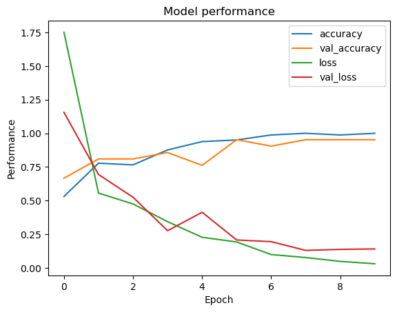
Figure left: Binary classification CNN model performance without dropout regularization Right: CNN model performance with dropout regularization
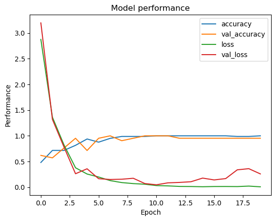
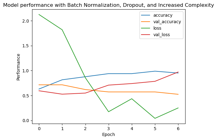
Figure left: Binary classification CNN model with 0.3 dropout regularization Right: CNN with batch regularization and early stopping
| Activation Function (Hidden layers) | Hidden Layers | Dropout Regularization (0.5) | Epochs | Validation Accuracy (%) | CV Error Rate (%) |
|---|---|---|---|---|---|
| Sigmoid | 1 | Yes | 10 | 67.24 | 1.12 |
| 2 | 54.31 | 1.69 | |||
| 3 | 24.14 | 2.34 | |||
| ReLU | 1 | Yes | 62.93 | 1.30 | |
| 2 | 36.21 | 1.99 | |||
| 3 | 12.93 | 2.38 | |||
| Leaky ReLU | 1 | Yes | 53.45 | 2.94 | |
| 2 | 57.76 | 1.82 | |||
| 3 | 44.83 | 1.97 | |||
| Tanh | 1 | Yes | 63.79 | 1.12 | |
| 2 | 55.17 | 1.42 | |||
| 3 | 46.55 | 1.79 | |||
| ReLU - CNN | 3 | No | 67.24 | 2.0 | |
| 4 | Yes | 68.97 | 1.1 | ||
| CNN - Class Weights | 4 | Yes | 69.83 | 1.01 | |
| 20 | 72.41 | 1.06 |
Figure Multi-class classification models performance metrics
Sigmoid Activation Function: With 1 hidden layer and dropout regularization, the model achieved a validation accuracy of 67.24%. Adding more hidden layers (2 and 3) resulted in a decrease in validation accuracy. with increasing CV error rates, indicating overfitting or inadequate learning.
ReLU Activation Function: The model with 1 hidden layer and dropout regularization achieved a validation accuracy of 62.93%, when the number of hidden layers was increased, there’s a significant drop in performance, with the model’s accuracy falling to ~ 12.93% and high CV error rates, indicating overfitting.
Leaky ReLU Activation Function: Unlike other models, increasing to 2 and 3 hidden layers showed a slight improvement in validation accuracy to 57.76% and 44.83%, but still had relatively high CV error rates. Tanh Activation Function: The model with 1 hidden layer and dropout regularization performed well with a validation accuracy of 63.79%. However, adding more hidden layers reduced the performance, with validation accuracy dropping to 55.17% and 46.55%, and increased CV error rates.
CNN with 3 hidden layers and no dropout gave a validation accuracy of 67.24% and a CV error rate of 2.0% only. CNN with Class Weights, 4 hidden layers and dropout achieved a validation accuracy of 68.97% and a CV error rate of 1.1%. Another configuration with class weights achieved a validation accuracy of 69.83% and a CV error rate of 1.01%. Extending the training to 20 epochs improved the performance further, with a validation accuracy of 72.41% and a CV error rate of 1.06%.

Confusion matrix with dropout regularization
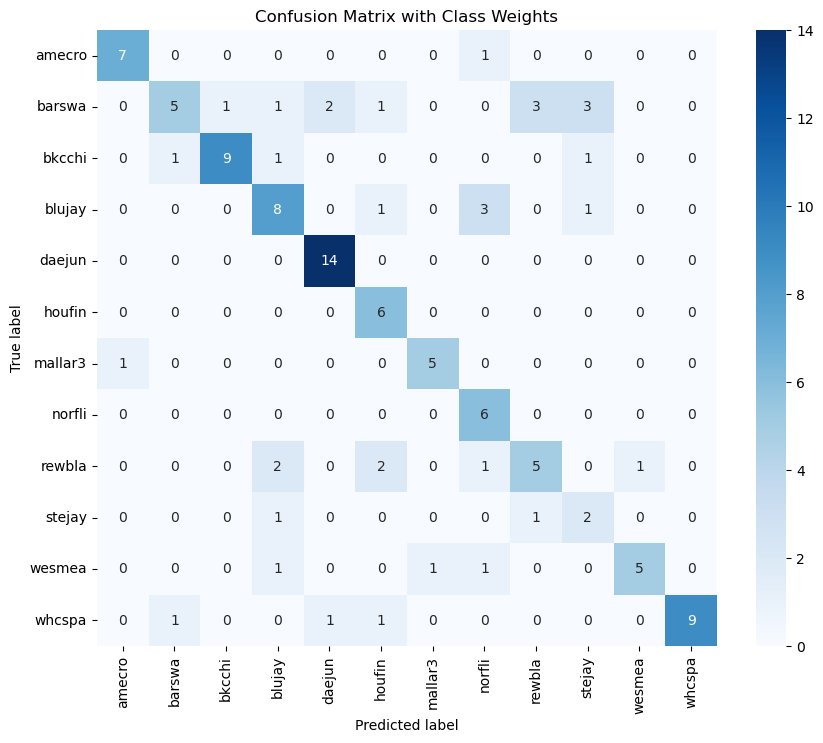
Confusion matrix with class weights and 10 epochs
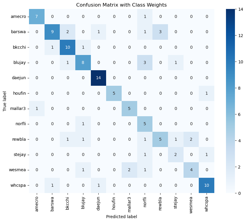
Confusion matrix with class weights and 20 epochs
As it is evident, there’s improvement in predictions when we used class weights, this was done because there was class imbalance in the dataset and it led to probabilities of solid 1s and 0s. The models also exhibit overfitting signs due to the imbalance in data. We tried many models and the most efficient were CNNs, although the highest accuracy was 72% for the multi-class classification model.
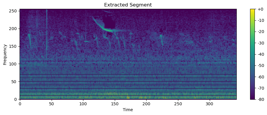
For external testing, when noise reduction was not used, the model struggled to predict the species and we saw 0s and 1s in probabilities. We have used 3 loud segments from the mp3 files and these are called segments. S1,S2,S3 are segments 1,2 and 3. With noise reduction, the model showed great performance. The probabilities can be seen in the table below.
| Species Name | Audio File 1 (S1) | Audio File 1 (S2) | Audio File 1 (S3) | Audio File 2 (S1) | Audio File 2 (S2) | Audio File 2 (S3) | Audio File 3 (S1) | Audio File 3 (S2) | Audio File 3 (S3) |
|---|---|---|---|---|---|---|---|---|---|
| American crow | 0.0342 | 0.0192 | 0.0640 | 0.5498 | 0.0006 | 0.0208 | 0.2306 | 0.0095 | 0.6532 |
| Barn swallow | 0.8346 | 0.0127 | 0.3962 | 0.0786 | 0.2246 | 0.4360 | 0.1700 | 0.0202 | 0.0229 |
| Black-capped chickadee | 0.0000 | 0.4753 | 0.3477 | 0.1460 | 0.0047 | 0.0298 | 0.0677 | 0.5501 | 0.3212 |
| Blue jay | 0.0153 | 0.0012 | 0.1311 | 0.0498 | 0.6698 | 0.0334 | 0.0010 | 0.0002 | 0.0002 |
| Dark-eyed junco | 0.0001 | 0.3376 | 0.0023 | 0.0000 | 0.0000 | 0.0009 | 0.0050 | 0.0811 | 0.0000 |
| House-finch | 0.0000 | 0.0087 | 0.0003 | 0.0000 | 0.0000 | 0.0000 | 0.0000 | 0.0359 | 0.0000 |
| Mallard | 0.0027 | 0.0032 | 0.0146 | 0.0001 | 0.0002 | 0.0002 | 0.0001 | 0.0007 | 0.0000 |
| Northern flicker | 0.0000 | 0.0033 | 0.0004 | 0.0000 | 0.0000 | 0.0000 | 0.0000 | 0.0001 | 0.0000 |
| Red-winged blackbird | 0.0348 | 0.0161 | 0.0126 | 0.1004 | 0.0047 | 0.0510 | 0.5219 | 0.3010 | 0.0003 |
| Stellar’s jay | 0.0657 | 0.0007 | 0.0004 | 0.0017 | 0.0031 | 0.0006 | 0.0026 | 0.0000 | 0.0000 |
| Western meadowlark | 0.0002 | 0.0729 | 0.0024 | 0.0001 | 0.0000 | 0.0001 | 0.0000 | 0.0001 | 0.0000 |
| White-crowned sparrow | 0.0126 | 0.0491 | 0.0279 | 0.0734 | 0.0923 | 0.4272 | 0.0011 | 0.0011 | 0.0021 |
Figure results of external testing - probabilities
The results show that audio files might have more than one species’s vocalization. Which is why we have ranked them based on their descending probabilities below.
| Audio File | Dominant Species |
|---|---|
| Audio File 1 | 1. Barn swallow |
| 2. Black-capped chickadee | |
| 3. Dark-eyed junco | |
| Audio File 2 | 1. Blue jay |
| 2. American crow | |
| 3. Barn swallow | |
| Audio File 3 | 1. American crow |
| 2. Black-capped chickadee | |
| 3. Red-winged blackbird |
Figure Dominant species based on aggregated probabilities for each audio file
Discussion
Overall, we explored various neural network architectures with varying functions and parameters. We saw models overfitting and underfitting under different parameters. CNNs have shown a stable performance across both classification problems. We have explored techniques like Batch Normalization and dropout regularization to make the learning process more efficient and reliable. When we notice class imbalance in the dataset, we use class weights to help the model generalize well. This showed significant difference in the model’s performance and that’s evident through the three confusion matrices shown in the computational results. As shown in the results table, especially for binary classification, we can see signs of overfitting where the model wasn’t learning well and achieving high test accuracy even though the training accuracy was low.
And running some of the neural networks with complex architecture took a lot of time. Multi-class classification took almost 8 mins but since the dataset size was not that large, the NNs didn’t take as much time and computational power as they’re expected to. The binary classification models took around 4 mins to train. Early stopping also helped us save time and make the model learn in a more efficient way.
The species that proved most challenging to predict were the House Finch, Mallard, and Northern Flicker, due to consistently low probabilities. Some species, like the Black-capped Chickadee and Blue Jay, or Stellar’s Jay and Red-winged Blackbird, showed potential confusion with one another as we can see in the confusion matrices. The dataset is also not large enough for this kind of bird identification task which requires more training data.
Other models like decision trees, support vector machines, and random forests can be used too. However, a neural network is more suitable for this kind of application because it learns complex data patterns very well compared to traditional models. Neural networks also have the advantage of being able to generalize well to unseen data, making them suitable for classification tasks such as this one.
Conclusion
In conclusion, the study focused on two different classification tasks: Binary Classification, Multi-Class Classification. The main goal was to classify different bird species based on their vocalizations. The study used various deep learning models such as CNN, Sequential CNN with different architectures and parameters along with dropout regularization and batch normalization techniques to combat overfitting. We evaluated their performance based on accuracy and loss metrics. We achieved commendable performance on both binary as well as multi-class classification tasks with such a limited dataset that had a potential class imbalance.
This research contributed to the understanding of classifying bird species based on audio recordings. Despite the challenges faced, the findings provide insights for future enhancements and optimizations in the field of bird species classification using neural networks. With further improvements and expanded datasets, it is possible to achieve more accurate and reliable classification results, thereby contributing to research and conservation efforts.
References
[1] Rao, R. (n.d.). Xeno-canto bird recordings extended [Data set]. Kaggle. Retrieved from https://www.kaggle.com/datasets/rohanrao/xeno-canto-bird-recordings-extended-a-m
[2] Laiolo, P. (2010). The emerging significance of bioacoustics in animal species conservation. Biological Conservation, 143(7), 1635-1645. https://doi.org/10.1016/j.biocon.2010.03.025.
[3] James, G., Witten, D., Hastie, T., Tibshirani, R., & Taylor, J. (2023). An Introduction to Statistical Learning with Applications in Python. (Original work published 2023) https://hastie.su.domains/ISLP/ISLP_website.pdf.download.html
[4] Bastian, M. (2019, October 11). Neural Network: The Dead Neuron. Towards Data Science. https://towardsdatascience.com/neural-network-the-dead-neuron-eaa92e575748